

Disclaimer:
The authors are solely responsible for the content of this report. Material included herein does not represent the opinion of the European Community, and the European Community is not responsible for any use that might be made of it.
Back to overview reports
Multivariate analysis was applied to bird data in order to explore the main patterns of spatial variation in wader and wildfowl community. In the Humber, bird species density was averaged over 5-year periods per sector (period 1=1975-1979, 2=1980-1984, 3=1985-1989, 4=1990-1995, etc) in order to account also for the general temporal variability (but reducing inter-annual fluctuations). For the Weser and Elbe, the analysis was performed on bird data averaged over a combination of estuarine zone, jurisdiction (north/south bank, Weser only) and 5-year period. Bird densities were forth root transformed and the Bray-Curtis similarity matrices were calculated before applying cluster analysis to highlight similarities in spatial-temporal distribution of different species in the studied estuaries. The general pattern in species distribution across estuarine zones was also investigated by using ordination analysis (Principal Coordinate analysis, PCO). Analysis of similarity (ANOSIM) between guilds and between sectors (in the Humber) and estuarine zones (in the Elbe and Weser) was carried out to test for statistical significance in the observed patterns.
Multivariate multiple linear regression analysis was performed on bird species data and on continuous explanatory variables in order to identify the main factors affecting the overall bird assemblage spatial-temporal distribution. The multivariate multiple regression full model (including all explanatory variables) was investigated by using distance-based redundancy analysis (dbRDA). DISTLM routine was also applied to identify the best subset of variables explaining wader data variability (best reduced model, selected by backward selection method using AIC criterion). Correlation analysis (Spearman’s) was carried out to identify the main relationships between species densities and environmental variables.
It should be noted that the datasets analysed (including data averages by sector/zone and 5-year period) have variable spatial and temporal coverage which might affect the analysis results. The dataset for the Humber (bird species densities and all the environmental variables) covers only sectors in the mesohalyne and polyhaline zones and includes 27 observations for waders (between 1990 and 2005) and 28 observations for wildfowl (between 1985 and 2005). The datasets for the Elbe cover all the salinity zones (from freshwater to polyhaline), including 68 observations for which both bird densities and habitat areas are available (between 1984 and 1998) and 92 observations for which both bird densities and water quality parameters are available (between 2004 and 2009). As the datasets on habitats and water quality parameters are not temporally overlapping, the analysis has been carried out separately for the two types of abiotic characteristics in this estuary. The dataset for the Weser for which both bird densities and habitat areas are available covers all the salinity zones (from freshwater to polyhaline), including 43 observations (between 1984 and 2003). In turn the dataset for which both bird densities and water quality parameters are available includes 92 observations (between 2004 and 2009) covering only the freshwater and oligohaline zone. As the datasets on habitats and water quality parameters are only marginally overlapping (between 1992 and 2003, with a total of 6 observations), the analysis has been carried out separately for the two types of abiotic characteristics also in this estuary.
Results
The cluster analysis distinguishes groups of species within wader and wildfowl assemblages mainly on the basis of their overall abundance, with the clusters shown in the upper part of the dendrograms (Figure 3.1) usually including the most abundant species found in the estuaries (e.g. Dunlin, Golden Plover, Lapwing, Oystercatcher, Curlew for waders; Shelduck, Wigeon, Mallard, Teal for wildfowl). There is a general agreement between the cluster analysis and the guilds classification for wildfowl only, as confirmed by the presence of a significant difference between wildfowl guilds in all the estuaries (Table 3.1). However, this is likely ascribed to the general higher abundances observed for all the species within the estuarine feeder and marsh associated guilds rather than to a common spatial distribution within the different estuaries. For example, the estuarine feeder species are widely distributed across the estuarine zones in the Elbe, whereas they show high densities in the polyhaline and mesohaline areas of the Weser and in the oligohaline and mesohaline areas of the Humber. In turn, the groupings of wader species identified by the cluster analysis seem not to agree with the guilds distinction, as confirmed by the absence of a significant difference between wader guilds in all the estuaries (Table 3.1). This might be ascribed to the fact that the considered guilds basically account for species depending on mud for feeding or roosting, hence these might not distinguish different uses at the spatial scale considered (among sectors) (e.g. different guilds distribution of birds feeding on mud might occur within a sector, along the shore height gradient, based on the prey availability and preferences, but this might not be evident when considering the sector as a whole and when comparing different sectors).
The ordination analysis applied to bird data in the different sectors/units (Figure 3.2) shows the main spatial-temporal differentiation in the wader and wildfowl assemblage distribution within each estuary. Data points in the ordination plots (i.e., observations by unit/sector by 5-year period) have been classified according to the salinity zone in order to obtain preliminary information on the degree of agreement of the species distribution with the salinity zonation of the estuaries. ANOSIM test has been carried out also between salinity zones in each estuary with this purpose (Table 3.2).
It’s clear from the analysis how spatial patterns dominate over temporal ones, resulting in clusters of samples from different periods within each sector/estuarine zone, and in higher distances between sector/zones samples than between temporal samples within each sector/zone in the ordination plot (Figure 3.2).
Table 3.1. ANOSIM results (R value and significance p-level) of comparisons between guilds distribution for waders and wildfowl in the Humber, Weser and Elbe estuaries (ns=not significant).
Table 3.2. ANOSIM results (R value and significance p-level) of comparisons of wader and wildfowl assemblage structure between salinity zones in the Humber, Weser and Elbe estuaries (ns=not significant).
*The estuarine bank (northern, SH or southern, NDS) was included in the analysis for the Elbe as a crossed factor in the analysis.
Back to top
What environmental factors should be considered in the design of a compensation scheme for waterbirds and their habitats?
What environmental variables are most important in determining minimizing or basic compensatory requirements for waterbirds?
What is important in establishing a zonation for estuaries?
What tools and guidance are available to minimise and mitigate disturbance to waterbirds?
Determinants of bird habitat use in TIDE estuaries
Table of content
- 1. SUMMARY
- 2. INTRODUCTION
- 3. STRUCTURE OF THE REPORT
- 4. DATA USED
- 5. GENERAL CHARACTERISTICS OF BIRD ASSEMBLAGES IN TIDE ESTUARIES
- 6. BIRD ASSEMBLAGES DISTRIBUTION AND RELATIONSHIP WITH ENVIRONMENTAL VARIABLES
- 6a. Humber
- 6b. Weser
- 6c. Elbe
- 7. SPECIES DISTRIBUTION MODELS
- 7a. Dunlin
- 7b. Redshank, Golden Plover and Bar-tailed Godwit
- 7c. Shelduck, Pochard and Brent Goose
- 8. DISCUSSION
- 9. CONCLUSIONS
- 9a. Analysis Conclusions
- 9b. Management Recommendations
- 9c. Recommendations for Future Studies
- 10. REFERENCES
- 11. APPENDIX 1
- 12. APPENDIX 2
- 13. APPENDIX 3
- 14. APPENDIX 4
13. Appendix 3
Details on the analysis and results on bird assemblages distribution and its relationship with environmental variables in TIDE estuaries
MethodsMultivariate analysis was applied to bird data in order to explore the main patterns of spatial variation in wader and wildfowl community. In the Humber, bird species density was averaged over 5-year periods per sector (period 1=1975-1979, 2=1980-1984, 3=1985-1989, 4=1990-1995, etc) in order to account also for the general temporal variability (but reducing inter-annual fluctuations). For the Weser and Elbe, the analysis was performed on bird data averaged over a combination of estuarine zone, jurisdiction (north/south bank, Weser only) and 5-year period. Bird densities were forth root transformed and the Bray-Curtis similarity matrices were calculated before applying cluster analysis to highlight similarities in spatial-temporal distribution of different species in the studied estuaries. The general pattern in species distribution across estuarine zones was also investigated by using ordination analysis (Principal Coordinate analysis, PCO). Analysis of similarity (ANOSIM) between guilds and between sectors (in the Humber) and estuarine zones (in the Elbe and Weser) was carried out to test for statistical significance in the observed patterns.
Multivariate multiple linear regression analysis was performed on bird species data and on continuous explanatory variables in order to identify the main factors affecting the overall bird assemblage spatial-temporal distribution. The multivariate multiple regression full model (including all explanatory variables) was investigated by using distance-based redundancy analysis (dbRDA). DISTLM routine was also applied to identify the best subset of variables explaining wader data variability (best reduced model, selected by backward selection method using AIC criterion). Correlation analysis (Spearman’s) was carried out to identify the main relationships between species densities and environmental variables.
It should be noted that the datasets analysed (including data averages by sector/zone and 5-year period) have variable spatial and temporal coverage which might affect the analysis results. The dataset for the Humber (bird species densities and all the environmental variables) covers only sectors in the mesohalyne and polyhaline zones and includes 27 observations for waders (between 1990 and 2005) and 28 observations for wildfowl (between 1985 and 2005). The datasets for the Elbe cover all the salinity zones (from freshwater to polyhaline), including 68 observations for which both bird densities and habitat areas are available (between 1984 and 1998) and 92 observations for which both bird densities and water quality parameters are available (between 2004 and 2009). As the datasets on habitats and water quality parameters are not temporally overlapping, the analysis has been carried out separately for the two types of abiotic characteristics in this estuary. The dataset for the Weser for which both bird densities and habitat areas are available covers all the salinity zones (from freshwater to polyhaline), including 43 observations (between 1984 and 2003). In turn the dataset for which both bird densities and water quality parameters are available includes 92 observations (between 2004 and 2009) covering only the freshwater and oligohaline zone. As the datasets on habitats and water quality parameters are only marginally overlapping (between 1992 and 2003, with a total of 6 observations), the analysis has been carried out separately for the two types of abiotic characteristics also in this estuary.
Results
The cluster analysis distinguishes groups of species within wader and wildfowl assemblages mainly on the basis of their overall abundance, with the clusters shown in the upper part of the dendrograms (Figure 3.1) usually including the most abundant species found in the estuaries (e.g. Dunlin, Golden Plover, Lapwing, Oystercatcher, Curlew for waders; Shelduck, Wigeon, Mallard, Teal for wildfowl). There is a general agreement between the cluster analysis and the guilds classification for wildfowl only, as confirmed by the presence of a significant difference between wildfowl guilds in all the estuaries (Table 3.1). However, this is likely ascribed to the general higher abundances observed for all the species within the estuarine feeder and marsh associated guilds rather than to a common spatial distribution within the different estuaries. For example, the estuarine feeder species are widely distributed across the estuarine zones in the Elbe, whereas they show high densities in the polyhaline and mesohaline areas of the Weser and in the oligohaline and mesohaline areas of the Humber. In turn, the groupings of wader species identified by the cluster analysis seem not to agree with the guilds distinction, as confirmed by the absence of a significant difference between wader guilds in all the estuaries (Table 3.1). This might be ascribed to the fact that the considered guilds basically account for species depending on mud for feeding or roosting, hence these might not distinguish different uses at the spatial scale considered (among sectors) (e.g. different guilds distribution of birds feeding on mud might occur within a sector, along the shore height gradient, based on the prey availability and preferences, but this might not be evident when considering the sector as a whole and when comparing different sectors).
The ordination analysis applied to bird data in the different sectors/units (Figure 3.2) shows the main spatial-temporal differentiation in the wader and wildfowl assemblage distribution within each estuary. Data points in the ordination plots (i.e., observations by unit/sector by 5-year period) have been classified according to the salinity zone in order to obtain preliminary information on the degree of agreement of the species distribution with the salinity zonation of the estuaries. ANOSIM test has been carried out also between salinity zones in each estuary with this purpose (Table 3.2).
It’s clear from the analysis how spatial patterns dominate over temporal ones, resulting in clusters of samples from different periods within each sector/estuarine zone, and in higher distances between sector/zones samples than between temporal samples within each sector/zone in the ordination plot (Figure 3.2).
Table 3.1. ANOSIM results (R value and significance p-level) of comparisons between guilds distribution for waders and wildfowl in the Humber, Weser and Elbe estuaries (ns=not significant).
| Humber | Weser | Elbe | |
| Waders | R=0.107 (ns) | R=0.050 (ns) | R=0.092 (ns) |
| Wildfowl | R=0.579 (p<0.001) | R=0.773 (p<0.001) | R=0.801 (p<0.001) |
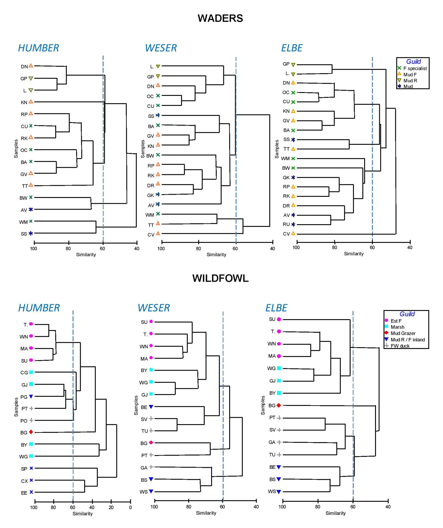
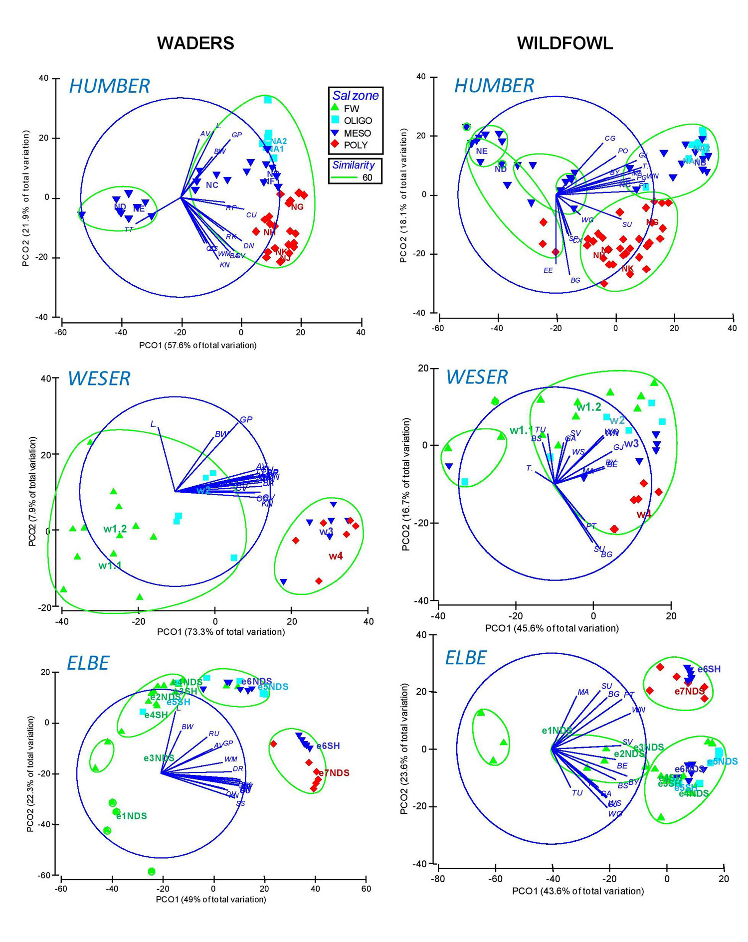
Table 3.2. ANOSIM results (R value and significance p-level) of comparisons of wader and wildfowl assemblage structure between salinity zones in the Humber, Weser and Elbe estuaries (ns=not significant).
| Humber | Weser | Elbe* | |
| Waders | R=0.390 (p<0.001) | R=0.725 (p<0.001) | R=0.184 (p<0.05) |
| Wildfowl | R=0.280 (p<0.001) | R=0.163 (p<0.05) | R=0.116 (ns) |
*The estuarine bank (northern, SH or southern, NDS) was included in the analysis for the Elbe as a crossed factor in the analysis.
Important to know
Reports / Measures / Tools
| Report: | Management measures analysis and comparison |
|---|
Management issues
How can management targets and monitoring strategies be set for waterbirds in compensatory areas?What environmental factors should be considered in the design of a compensation scheme for waterbirds and their habitats?
What environmental variables are most important in determining minimizing or basic compensatory requirements for waterbirds?
What is important in establishing a zonation for estuaries?
What tools and guidance are available to minimise and mitigate disturbance to waterbirds?